This tutorial will cover a boilerplate RNAseq analysis using Salmon psuedo-alignment of illumina generated paired-end reads to the Arabidopsis thaliana transcriptome. While running this tutorial line-by-line can be a useful to learn the various data transformation steps, some things, such as for loops and variable storage are a little awkward to run line-by-line in a terminal. Therefore, here is a link to the bash script and the R script to make it a little easier to follow along.

Reads are from a publically available dataset for testing the transcriptomic response of Arabidopsis thaliana to dopamine.

We will cover:

Data cleaning (shell and other tools)
Alignment of reads (Salmon)
Statistical analysis of alignment data (R and edgeR)

The data cleaning step of this tutorial is broadly applicable to any workflow. Once the data is cleaned, there are many ways to proceed with alignment. Here we use Salmon, a very efficient alignment program.

Setting up your environment

This tutorial uses open-source bioinformatics tools and R.

Installing the tools

We will install our tools using conda. I have included a conda environment yml, to get things up and running quickly. Skip this step if these programs are already available to you or if you wish to install them nativly.

If you go the conda route, download the conda environment yml and install the environment.

conda env create -f rnaSalmon.yml

then activate the environment…

conda activate rnaSalmon

packages include:

R

If you don’t have R and R-studio installed, get it installed.

one last thing to download…

Finally, there is a python script from the Harvard Bioinformatics team which is useful here. Download the python script and place it in the working directory you have chosen to use for this tutorial.

FilterUncorrectabledPEfastq.py

Variables

{cName}{i}, {tName}{i} and {threads}

If you wish to make all of this code run without editing it, you can simply set the $cName, $tName and $threads string variables in your bash session. These variables are for your control read names, treatment read names and the number of threads you want to use for the analysis. Here, we will simply cName our data cDA2 and tName tDA2. The thread number is set to 20 here, for use on 24 core machines to give you some headroom for using the computer while the analysis is running.

cName='cDA2'
tName='tDA2'
threads='20'

reps

Set this variable as an array of your replicate measurements. For nearly every command in the following section, we will be using a for loop to run each command on all of the replicates. In our example, we will have 3.

declare -a reps=("R1" "R2" "R3")

Data Acquisition & Cleaning

Get data (or use your own)

First we need to download our data. For this we will use Sequence Reach Archive Tools.

fasterq-dump --fasta --split-files SRX18321587
mv SRX18321587_1* cDA2_R1_1.fq
mv SRX18321587_2* cDA2_R1_2.fq
fasterq-dump --fasta --split-files SRX18321588
mv SRX18321588_1* cDA2_R2_1.fq
mv SRX18321588_2* cDA2_R2_2.fq
fasterq-dump --fasta --split-files SRX18321591
mv SRX18321591_1* cDA2_R3_1.fq
mv SRX18321591_2* cDA2_R3_2.fq
fasterq-dump --fasta --split-files SRX18321595
mv SRX18321595_1* tDA2_R1_1.fq
mv SRX18321595_2* tDA2_R1_2.fq
fasterq-dump --fasta --split-files SRX18321596
mv SRX18321596_1* tDA2_R2_1.fq
mv SRX18321596_2* tDA2_R2_2.fq
fasterq-dump --fasta --split-files SRX18321597
mv SRX18321597_1* tDA2_R3_1.fq
mv SRX18321597_2* tDA2_R3_2.fq
gzip *.fq

Clean Data

Assess the quality of the raw data using FASTQC (How to read and interperate FastQC reports)

mkdir qcRaw

for i in "${reps[@]}"
do
    fastqc --threads $threads --outdir ./qcRaw ./${cName}_{i}_1.fq.gz
    fastqc --threads $threads --outdir ./qcRaw ./${cName}_{i}_2.fq.gz
    fastqc --threads $threads --outdir ./qcRaw ./${tName}_{i}_1.fq.gz
    fastqc --threads $threads --outdir ./qcRaw ./${tName}_{i}_2.fq.gz
done

Run rCorrector

rCorrector will repair read pairs which are low quality.

mkdir ./rCorr

for i in "${reps[@]}"
do
    rcorrector \
        -ek 20000000000 \
        -t $threads \
        -od ./rCorr \
        -1 ../${cName}_{i}_1.fq \
        -2 ../${cName}_{i}_2.fq
    rcorrector \
        -ek 20000000000 \
        -t $threads \
        -od ./rCorr \
        -1 ../${tName}_{i}_1.fq \
        -2 ../${tName}_{i}_2.fq
done

cd rCorr
for i in "${reps[@]}"
do
    python ../FilterUncorrectabledPEfastq.py -1 ${cName}_{i}_1.cor.fq -2 ${cName}_{i}_2.cor.fq -s ${cName}_{i}
    python ../FilterUncorrectabledPEfastq.py -1 ${tName}_{i}_1.cor.fq -2 ${tName}_{i}_2.cor.fq -s ${tName}_{i}
done

Remove unfixable reads

for i in "${reps[@]}"
do
    trim_galore \
        -j 8 \
        --paired \
        --retain_unpaired \
        --phred33 \
        --output_dir ./trimmed_reads \
        --length 36 \
        -q 5 \
        --stringency 1 \
        -e 0.1
        unfixrm_${cName}_{i}_1.cor.fq unfixrm_${cName}_{i}_2.cor.fq
    trim_galore \
        -j 8 \
        --paired \
        --retain_unpaired \
        --phred33 \
        --output_dir ./trimmed_reads \
        --length 36 \
        -q 5 \
        --stringency 1 \
         -e 0.1 \
         unfixrm_${tName}_{i}_1.cor.fq unfixrm_${tName}_{i}_2.cor.fq
done

Remove reads originating from ribsomal RNA

Most modern RNAseq library prep methods are very good at minimizing rRNA contamination, but there is always some.

To correct for this, we are going to map our reads to the SILVA rRNA blacklist, and output those reads which don’t align. This will remove rRNA contamination.

First, lets create a directory to keep things organized

mkdir riboMap   
cd riboMap

Download the SILVA rRNA blacklists for the Large and Small subunits, which we will subsequently use to clean our reads of rRNA contamination.

wget "https://www.arb-silva.de/fileadmin/silva_databases/release_138_1/Exports/SILVA_138.1_LSURef_NR99_tax_silva.fasta.gz"
wget "https://www.arb-silva.de/fileadmin/silva_databases/release_138_1/Exports/SILVA_138.1_SSURef_NR99_tax_silva.fasta.gz"

Unzip the files, concatonate them and replace “U” in the fasta sequences with “T”

gunzip ./*
cat SILVA_138.1_LSURef_NR99_tax_silva.fasta > SILVArRNAdb.fa.temp
cat SILVA_138.1_SSURef_NR99_tax_silva.fasta > SILVArRNAdb.fa.temp
sed '/^[^>]/s/U/T/g' SILVArRNAdb.fa.temp > SILVAcDNAdb.fa
rm SILVArRNAdb.fa.temp

Align the reads using Bowie2 to the rRNA blacklist. Those reads which do not align to the blacklist will be output as clean_{cName}{i}_1.fq.gz and clean{cName}_{i}_2.fq.gz

for i in "${reps[@]}"
do
    bowtie2 --quiet --very-sensitive-local --phred33  \
        -x SILVAcDNAdb \
        -1 ../rCorr/trimmed_reads/unfixrm_${cName}_{i}_1.cor_val_1.fq \
        -2 ../rCorr/trimmed_reads/unfixrm_${cName}_{i}_2.cor_val_2.fq \
        --threads $threads \
        --met-file ${cName}_{i}_bowtie2_metrics.txt \
        --al-conc-gz blacklist_paired_aligned_${cName}_{i}.fq.gz \
        --un-conc-gz clean_${cName}_{i}.fq.gz  \
        --al-gz blacklist_unpaired_aligned_${cName}_{i}.fq.gz \
        --un-gz blacklist_unpaired_unaligned_${cName}_{i}.fq.gz
    bowtie2 --quiet --very-sensitive-local --phred33  \
        -x SILVAcDNAdb \
        -1 ../rCorr/trimmed_reads/unfixrm_${tName}_{i}_1.cor_val_1.fq \
        -2 ../rCorr/trimmed_reads/unfixrm_${tName}_{i}_2.cor_val_2.fq \
        --threads $threads \
        --met-file ${tName}_{i}_bowtie2_metrics.txt \
        --al-conc-gz blacklist_paired_aligned_${tName}_{i}.fq.gz \
        --un-conc-gz clean_${tName}_{i}.fq.gz  \
        --al-gz blacklist_unpaired_aligned_${tName}_{i}.fq.gz \
        --un-gz blacklist_unpaired_unaligned_${tName}_{i}.fq.gz
done

Navigate to your primary working directory, and create a directory for your FastQC outputs of your cleaned data

cd ..
mkdir ./qcClean
cd ./qcClean

Reasses the quality of your data using FastQC.

for i in "${reps[@]}"
do
    fastqc --threads $threads --outdir ./ ../riboMap/clean_${cName}_{i}_1.fq
    fastqc --threads $threads --outdir ./ ../riboMap/clean_${cName}_{i}_2.fq
    fastqc --threads $threads --outdir ./ ../riboMap/clean_${tName}_{i}_1.fq
    fastqc --threads $threads --outdir ./ ../riboMap/clean_${tName}_{i}_2.fq
done

At this point, your data should be in good shape.

Generate Count Data Using Salmon

Make Arabidopsis thaliana index

First, we need to download the Arabidopsis thaliana reference transcriptome and index it for Salmon. There are a number of options for indexing in Salmon (docs). You may notice the documentation recommends running in decoy-aware mode. This can be safely ignored in Arabidopsis, as the reference transcripome is very good. For organisms with less robust reference transcriptomes decoy awareness can avoid spurious mapping of your reads (to, for example transcribed psuedogenes).

wget -O athal.fa.gz "ftp://ftp.ensemblgenomes.org/pub/plants/release-28/fasta/arabidopsis_thaliana/cdna/Arabidopsis_thaliana.TAIR10.28.cdna.all.fa.gz"
salmon index -t athal.fa.gz -i athal_index

Run Salmon

Soft-link your cleaned FQ files. Not really necissary, but makes the run command tidier.

mkdir salmon_out
cd salmon_out
for i in "${reps[@]}"
do
    ln -s ../riboMap/clean_${cName}_{i}_1.fq ./clean_${cName}_{i}_1.fq
    ln -s ../riboMap/clean_${cName}_{i}_2.fq ./clean_${cName}_{i}_2.fq
    ln -s ../riboMap/clean_${cName}_{i}_1.fq ./clean_${tName}_{i}_1.fq
    ln -s ../riboMap/clean_${cName}_{i}_2.fq ./clean_${tName}_{i}_2.fq
    salmon quant \
        -i ../athal_index \
        -l A -1 clean_${cName}_{i}_1.fq \
        -2 clean_${cName}_{i}_2.fq \
        --gcBias \
        -p 20 \
        --validateMappings \
        -o ${cName}_{i}_transQ
    salmon quant \
        -i ../athal_index \
        -l A \
        -1 clean_${tName}_{i}_1.fq \
        -2 clean_${tName}_{i}_2.fq \
        --gcBias \
        -p 20 \
        --validateMappings \
        -o ${tName}_{i}_transQ
done

Statistical Analysis of Count Data Using R

First we need to download the gene features file for the Arabidopsis transcriptome. This will allow the production of gene-level abundence estemates using tximport. This step dramatically simplifies analysis and the interpritation of results.

wget "https://www.arabidopsis.org/download_files/Genes/TAIR10_genome_release/TAIR10_gff3/TAIR10_GFF3_genes.gff"

Now it’s time to leave the bash environment and fire up R studio.

install needed libraries and load them up

setwd("./")
if (!require("BiocManager", quietly = TRUE))
    install.packages("BiocManager")
BiocManager::install(version = "3.17")

BiocManager::install("edgeR")
BiocManager::install("tximport")

library('edgeR')
library('tximport')

make TxDB for TAIR

gtffile <- "./TAIR10_GFF3_genes.gff"
file.exists(gtffile)
txdb <- makeTxDbFromGFF(gtffile, format = "gff3", circ_seqs = character())
k <- keys(txdb, keytype = "TXNAME")
tx2gene <- select(txdb, k, "GENEID", "TXNAME")
write.csv(tx2gene, file = "./TAIR10tx2gene.gencode.v27.csv")
head(tx2gene)

Import data using tximport

#Read in tx2gene database
tx2gene <- read_csv("./TAIR10tx2gene.gencode.v27.csv")

Read in sample list (file names and factors)

In order to set up the analysis, we need to create a dataframe containing our experimental design. We have two conditions with three replicates each.

samples <- data.frame(samples = c('cDA2_R1', 'cDA2_R2', 'cDA2_R3', 'tDA2_R1', 'tDA2_R2', 'tDA2_R3'),
                      condition = rep(LETTERS[1:2], each = 3))

head(samples)

Retrieve file paths for salmon .sf files

files <- file.path(paste0(samples$samples,"_quant.sf") 
names(files) <- paste0("sample", 1:6)
all(file.exists(files))
head(files)

Import salmon .sf files, and summarize to gene using tx2gene database

txi <- tximport(files, type = "salmon", tx2gene = tx2gene)

Prep Data for EdgeR

cts <- txi$counts
head(cts)

Use edgeR function DGEList to make read count list

d <- DGEList(counts=cts,group=factor(samples$condition))
head(d)

Data Filtering

dim(d)
d.full <- d # keep in case things go awry
head(d$counts)
head(cpm(d))
apply(d$counts,2,sum)

Trim lowly-abundant genes. cpm number can be changed based on library size, and detected tags.

keep <- rowSums(cpm(d)>100) >= 2
keep
d <- d[keep,]
dim (d)
d$samples$lib.size <- colSums(d$counts)
d$samples

Normalize data

d <- calcNormFactors(d, logratioTrim = 0)
d

Run sample-wise PCA, to check sample grouping

plotMDS(d, method="bcv", col=as.numeric(d$samples$group))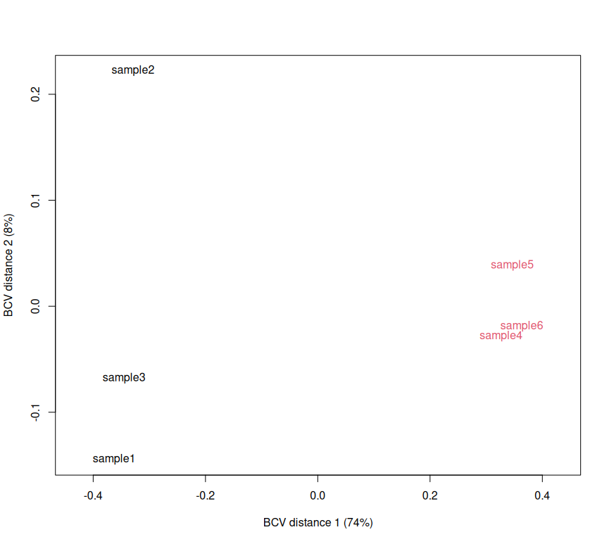

Estimate and plot dispersion of tags vs Log~2~ Fold Change (FC)

d1 <- estimateCommonDisp(d, verbose=T)
names(d1)

d1 <- estimateTagwiseDisp(d1)
names(d1)
plotBCV(d1)

Make design matrix; estimate common dispersion and trended dispersion

design.mat <- model.matrix(~ 0 + d$samples$group)
colnames(design.mat) <- levels(d$samples$group)
d2 <- estimateGLMCommonDisp(d,design.mat)
d2 <- estimateGLMTrendedDisp(d2,design.mat, method="power")

d2 <- estimateGLMTagwiseDisp(d2,design.mat)
plotBCV(d2)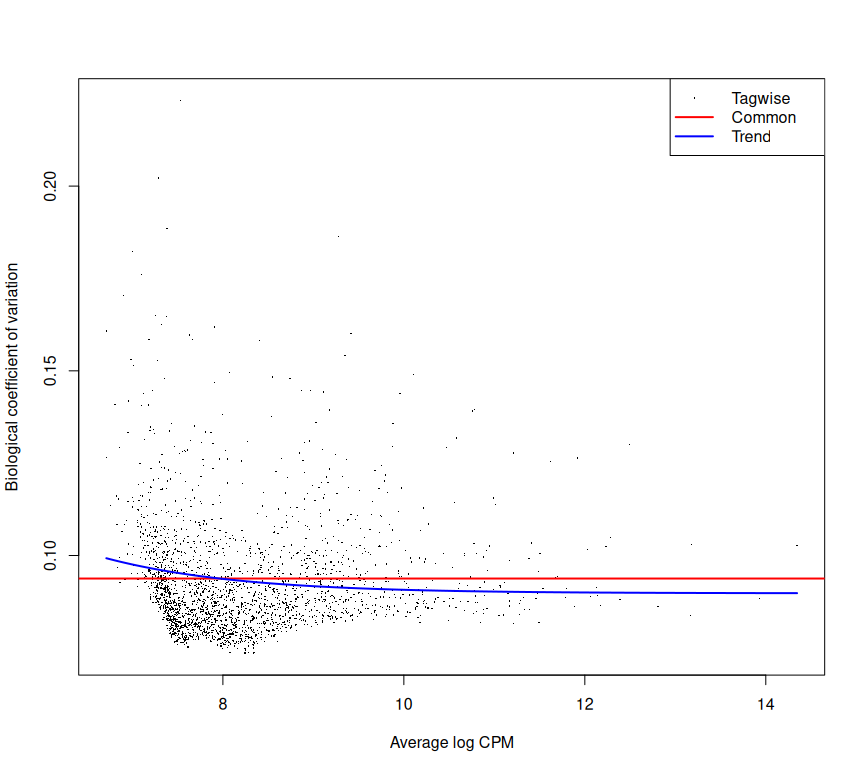

Run Fishers Exact Test, comparing the control vs the treatment

et12 <- exactTest(d1, pair=c(1,2)) # compare groups 1 and 2

Check out your top DEGs.

topTags(et12,n=100)

Identify significant DE genes (P < 0.05) and adjust for multiple comparisons

de1 <- decideTestsDGE(et12, adjust.method="BH")
summary(de1)

differentially expressed tags from the naive method in d1, make volcano plot

de1tags12 <- rownames(d1)[as.logical(de1)] 
plotSmear(et12, de.tags=de1tags12)
abline(h = c(-2, 2), col = "blue")
design.mat
fit <- glmFit(d2, design.mat)
summary(de1)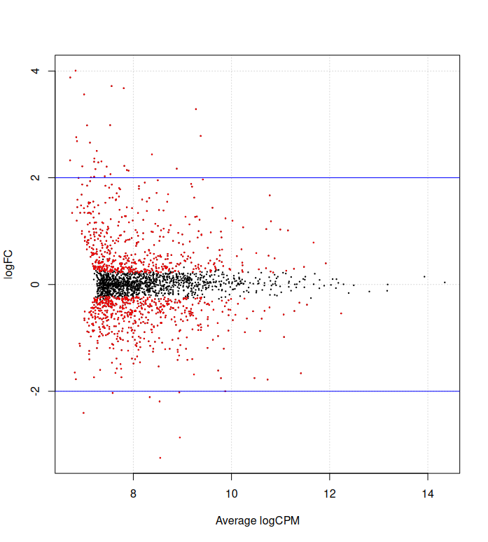

Save results in a CSV.

DE <- topTags(et12,n=5000)
as.data.frame(DE)
write.csv(DE, DA2H_DEGs.csv))